Getting Started with randomForestSGT
Hemant Ishwaran (hemant.ishwaran@gmail.com)
Min Lu (luminwin@gmail.com)
Udaya B. Kogalur (ubk@kogalur.com)
2026-05-14

Overview
The randomForestSGT package implements Super
Greedy Trees (SGTs), a flexible decision tree method for
regression [1]. Unlike standard CART
models, which rely on univariate splits, SGTs adaptively fit
lasso-penalized parametric models at each node, enabling rich
multivariate geometric cuts—such as hyperplanes, ellipsoids, and
higher-order surfaces.
These cuts provide greater flexibility in partitioning the feature space while retaining the interpretability of decision trees. The trees are grown greedily by maximizing empirical risk reduction using a best-split-first (BSF) strategy.
The package also supports: - Variable selection via importance
scoring - Filtering and dimension reduction using tune.hcut
- Robust handling of high-dimensional settings
How Super Greedy Trees Work
SGTs perform splitting by fitting a lasso-penalized model locally at
each node. The geometry of the split is determined by the
hcut parameter:
-
hcut = 0: Axis-aligned split (like CART) -
hcut = 1: Hyperplane cut (lasso linear model) -
hcut = 2–7: Curved and interaction-based cuts (e.g., ellipsoids, higher-order terms)
Coordinate descent is used for efficient model fitting, and cross-validation is applied to select the regularization parameter. The trees are grown sequentially by greedily selecting splits that maximize empirical risk reduction.
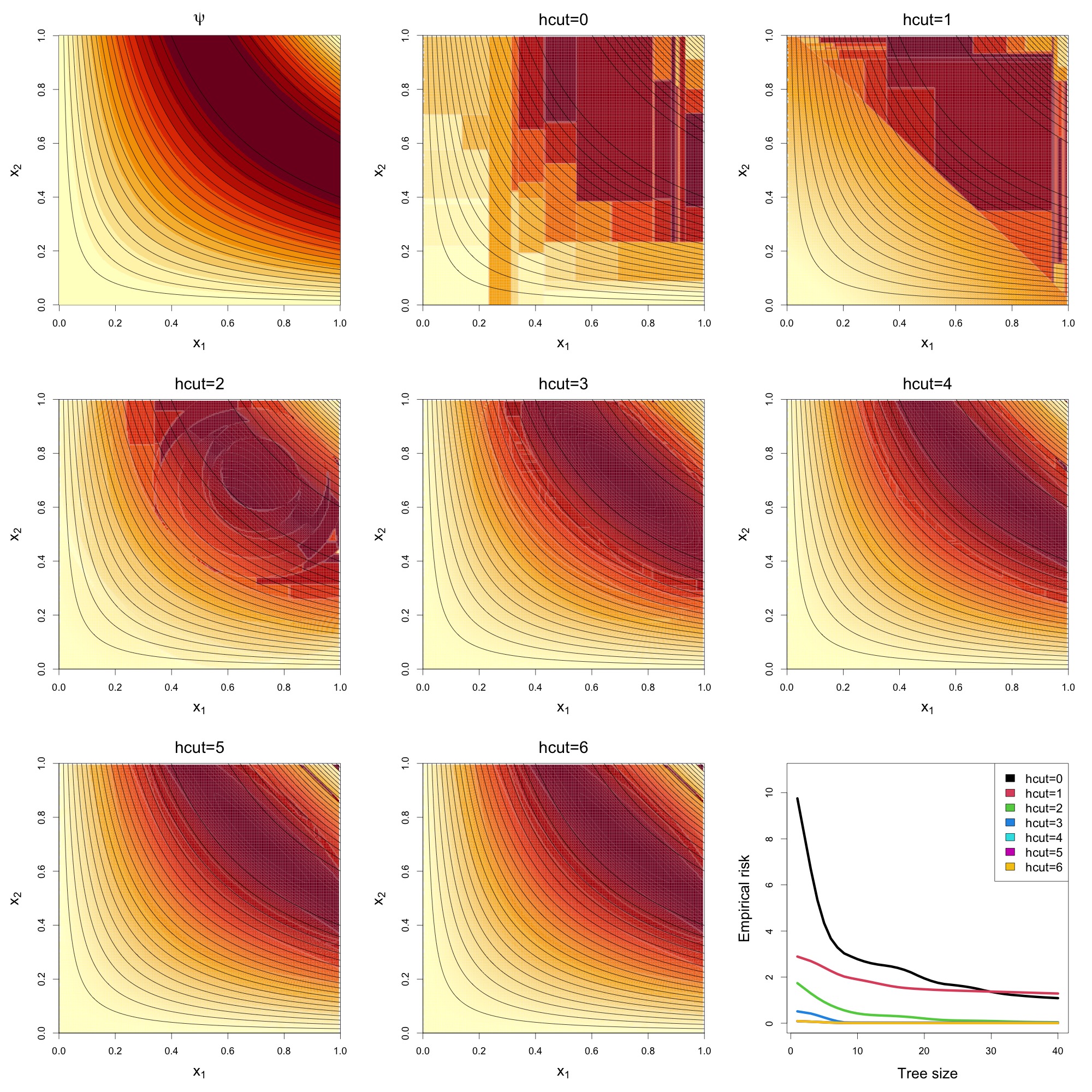
The above
figure presents results from a nonlinear simulation involving two
informative variables and 1,000 noise variables, under varying
hcut values. The top-left panel shows the true regression
surface
as a function of the two signal variables
.
The remaining panels (arranged left to right, top to bottom) display the
predicted surfaces from Super Greedy Trees (SGTs) with increasing
hcut values.
The hcut = 0 model, equivalent to standard CART,
produces piecewise constant predictions with axis-aligned splits.
Performance improves noticeably at hcut = 1, where oblique
(hyperplane-based) splits are introduced. As hcut increases
further, allowing for ellipsoidal and higher-order geometric cuts, the
predicted surfaces more closely approximate the true function.
The bottom-right panel plots empirical risk against tree size. Models
with hcut = 4, 5, and 6 achieve
rapid convergence to near-zero risk, demonstrating the advantage of
incorporating more flexible geometric partitions in high-dimensional
settings.
Quick Start with Quick Installation
Install the package using:
install.packages("randomForestSGT", repos = "https://cran.r-project.org")

# another way
install.packages("devtools")
devtools::install_github("kogalur/randomForestSGT")
Then load the package:
Examples
1. Boston Housing (regression)
data(BostonHousing, package = "mlbench")

# Default call
print(rfsgt(medv ~ ., BostonHousing))

                         Sample size: 506
                    Tree sample size: 320
                     Number of trees: 100
                   Average tree size: 67.94
                   Average node size: 4.723663
              Total no. of variables: 13
                              Family: regr
                           Splitrule: sg.regr
                                hcut: 1
                      hcut-dimension: 13
                       OOB R-squared: 0.8560169
         OOB standardized error rate: 0.1439831
                      OOB error rate: 12.17906

# Variable importance
sort(vimp.rfsgt(medv ~ ., BostonHousing))

       zn     indus       age      chas       rad       nox       tax         b       dis
0.2372256 0.4147085 0.5988148 0.8562534 1.1593113 1.3280123 1.5467381 1.5954471 1.8550349
  ptratio      crim        rm     lstat
2.7490414 4.9373395 6.0965162 9.9842085


# Using hcut = 0 (axis-aligned, like random forest)
print(rfsgt(medv ~ ., BostonHousing, hcut = 0))

                         Sample size: 506
                    Tree sample size: 320
                     Number of trees: 100
                   Average tree size: 66.7
                   Average node size: 4.815605
              Total no. of variables: 13
                              Family: regr
                           Splitrule: cart.regr
                                hcut: 0
                      hcut-dimension: 13
                       OOB R-squared: 0.8596718
         OOB standardized error rate: 0.1403282
                      OOB error rate: 11.8699


print(rfsgt(medv ~ ., BostonHousing, hcut = 0, nodesize = 1))

# Using hcut = 1 with smaller nodes
print(rfsgt(medv ~ ., BostonHousing, nodesize = 1))

                         Sample size: 506
                    Tree sample size: 320
                     Number of trees: 100
                   Average tree size: 200
                   Average node size: 1.6
              Total no. of variables: 13
                              Family: regr
                           Splitrule: cart.regr
                                hcut: 0
                      hcut-dimension: 13
                       OOB R-squared: 0.8833915
         OOB standardized error rate: 0.1166085
                      OOB error rate: 9.863532
2. Tuning hcut with Pre-filtering
# Simulate data
n <- 100
p <- 50
noise <- matrix(runif(n * p), ncol = p)
dta <- data.frame(mlbench:::mlbench.friedman1(n, sd = 0), noise = noise)

# Tune hcut
f <- tune.hcut(y ~ ., dta, hcut = 3)

# Use tuned hcut
print(rfsgt(y ~ ., dta, filter = f))

                         Sample size: 100
                    Tree sample size: 63
                     Number of trees: 100
                   Average tree size: 2.53
                   Average node size: 26.1975
              Total no. of variables: 4
                              Family: regr
                           Splitrule: sg.regr
                                hcut: 3
                      hcut-dimension: 9
                       OOB R-squared: 0.8344489
         OOB standardized error rate: 0.1655511
                      OOB error rate: 4.472403


# Override with specific hcut values
print(rfsgt(y ~ ., dta, filter = use.tune.hcut(f, hcut = 1)))

                         Sample size: 100
                    Tree sample size: 63
                     Number of trees: 100
                   Average tree size: 2.91
                   Average node size: 23.3835
              Total no. of variables: 4
                              Family: regr
                           Splitrule: sg.regr
                                hcut: 1
                      hcut-dimension: 4
                       OOB R-squared: 0.7943619
         OOB standardized error rate: 0.2056381
                      OOB error rate: 5.555361

print(rfsgt(y ~ ., dta, filter = use.tune.hcut(f, hcut = 2)))

                         Sample size: 100
                    Tree sample size: 63
                     Number of trees: 100
                   Average tree size: 2.7
                   Average node size: 24.885
              Total no. of variables: 4
                              Family: regr
                           Splitrule: sg.regr
                                hcut: 2
                      hcut-dimension: 6
                       OOB R-squared: 0.7829602
         OOB standardized error rate: 0.2170398
                      OOB error rate: 5.86338

print(rfsgt(y ~ ., dta, filter = use.tune.hcut(f, hcut = 3)))

                         Sample size: 100
                    Tree sample size: 63
                     Number of trees: 100
                   Average tree size: 2.58
                   Average node size: 25.6725
              Total no. of variables: 4
                              Family: regr
                           Splitrule: sg.regr
                                hcut: 3
                      hcut-dimension: 9
                       OOB R-squared: 0.8325974
         OOB standardized error rate: 0.1674026
                      OOB error rate: 4.522421
3. High-Dimensional Example with Variable Selection
# Simulate big-p-small-n setting
n <- 50
p <- 500
d <- data.frame(y = rnorm(n), x = matrix(rnorm(n * p), n))

# Variable selection via vimp
sort(vimp.rfsgt(y ~ ., d))

         x.1          x.2          x.4          x.5          x.6          x.7          x.9
0.0000000000 0.0000000000 0.0000000000 0.0000000000 0.0000000000 0.0000000000 0.0000000000
        x.10         x.15         x.16         x.17         x.18         x.19         x.20
0.0000000000 0.0000000000 0.0000000000 0.0000000000 0.0000000000 0.0000000000 0.0000000000
        x.23         x.24         x.27         x.29         x.30         x.31         x.34
0.0000000000 0.0000000000 0.0000000000 0.0000000000 0.0000000000 0.0000000000 0.0000000000

...

       x.445        x.346        x.313         x.91         x.39          x.8        x.195
0.0553205505 0.0607216646 0.0621489737 0.0667036813 0.0693496268 0.0711170419 0.0721632053
       x.121          x.3        x.370        x.457        x.105        x.350        x.156
0.0734905948 0.0735413342 0.0738475792 0.0762562215 0.0771366042 0.0813055104 0.0830835468
       x.249         x.33        x.255        x.206         x.37         x.77        x.402
0.0941898189 0.1275729727 0.1368649275 0.1382354223 0.1409270698 0.1766264978 0.1857151320
       x.227        x.148        x.179
0.2766907432 0.2898293950 0.6140237278


# Variable filtering using internal methods
filter.rfsgt(y ~ ., d, method = "conserve")

[1] "x.148" "x.156" "x.179" "x.206" "x.227" "x.402" "x.408"
What’s Next?
- Use
?rfsgtand?vimp.rfsgtto explore all arguments and options - Apply
tune.hcutfor automated dimension reduction - Use filtering for stability in high-dimensional data
- Try
hcut = 0for fast axis-aligned splits; use higherhcutfor richer geometry
Cite this vignette as
H. Ishwaran, M. Lu, and
U. B. Kogalur. 2025. “randomForestSGT: getting started with
randomForestSGT vignette.” http://www.randomforestsgt.org/articles/getstarted.html.
@misc{LuGettingStartedsgt,
    author = "Hemant Ishwaran and Min Lu and Udaya B. Kogalur",
    title = {{randomForestSGT}: getting started with {randomForestSGT} vignette},
    year = {2025},
    url = {http://www.randomforestsgt.org/articles/getstarted.html},
    howpublished = "\url{http://www.randomforestsgt.org/articles/getstarted.html}",
    note = "[accessed date]"
}